Kinetics Analysis of Underwater Gliders

Introduction

In our previous post on Kinematics, we built the mathematical bridge that connects a vehicle’s body-frame velocities to its position and orientation in the world. We answered the question: “Given the vehicle’s velocity, where is it going?” Now, we turn to the other half of the dynamics puzzle: Kinetics.

Kinetics is the study of the forces and moments that cause motion. It answers the fundamental question: “Given the forces acting on the vehicle, how will its velocity change?” This is the realm of Newton’s second law \(F=ma\) and its rotational equivalent.

However, applying these simple laws to a complex 6-DOF marine vehicle is not straightforward. The laws are defined in an idealized, non-accelerating inertial frame, but our vehicle operates in a rotating, body-fixed frame. This post will systematically walk through the process of translating these fundamental physical laws into a practical, complete 6-DOF rigid-body kinetic model, forming the core of any vehicle’s GNC system (Guidance, Navigation, and Control System).

1. What is Kinetics?

The study of motion, dynamics, is elegantly split into two parts:

• Kinematics: The geometry of motion, describing position and velocity without regard for forces. This was the focus of our last article.
• Kinetics: The cause of motion, relating the forces and moments acting on a body to its resulting accelerations.

In short: \(dynamics = kinematics + kinetics\). This article is dedicated to the latter. Our goal is to derive the famous rigid-body equation of motion:

This equation describes how the total external forces and moments, \(\tau_{RB}\), generate linear and angular accelerations, \(\dot{\nu}\).

2. The Cast of Characters: Frames, Points, and Velocities

Before we dive into the laws of motion, let’s re-establish our key reference frames and points, which are crucial for the derivation.

• North-East-Down (NED) Frame {n}: Our local navigation frame, which we approximate as an inertial frame. This is a crucial assumption, as Newton’s laws are only valid in a non-accelerating, non-rotating frame.
• BODY Frame {b}: A frame fixed to the vehicle, with its origin at a convenient point, \(O_b\). This frame rotates and translates with the vehicle, making it non-inertial.
• Coordinate Origin (CO): The origin \(O_b\) of the BODY frame {b}. This is a fixed point on the vehicle, often its geometric center. It’s the reference point for our final equations.
• Center of Gravity (CG): The point where the total gravitational force acts. Newton’s laws are naturally formulated about this point. The position of the CG relative to the CO is given by the vector \(r_{bg}^b\).

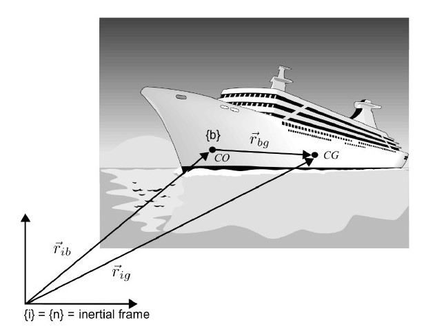
We use the standard SNAME notation for our state vectors:

• Generalized velocity in BODY {b}: \(\nu = [u, v, w, p, q, r]^T\)
• Generalized force in BODY {b}: \(\tau_{RB} = [X, Y, Z, K, M, N]^T\)

Our task is to find the matrices \(M_{RB}\) (Rigid-Body Mass) and \(C_{RB}(\nu)\) (Rigid-Body Coriolis and Centripetal) that govern the relationship between these vectors.

3. The Golden Standard: Newton-Euler Equations in an Inertial Frame

All of classical dynamics is built upon the Newton-Euler equations. These laws provide the “ground truth” for motion but are only valid under two strict conditions:

1. They must be expressed in an inertial frame (our NED frame {n}).
2. They must be formulated with respect to the body’s Center of Gravity (CG).

Let’s state them formally.

• Newton’s Second Law (Linear Motion): The rate of change of linear momentum equals the sum of external forces. \(\frac{d}{dt} (m v_{ig}) \bigg|_i = f_g\) where \(m\) is the mass, \(v_{ig}\) is the velocity of the CG in the inertial frame, and \(f_g\) is the total force acting on the CG.

• Euler’s Law (Angular Motion): The rate of change of angular momentum about the CG equals the sum of external moments about the CG. \(\frac{d}{dt} (h_g) \bigg|_i = m_g\) where \(h_g = I_g \omega_{ib}\) is the angular momentum, \(I_g\) is the inertia tensor about the CG, \(\omega_{ib}\) is the angular velocity of the body in the inertial frame, and \(m_g\) is the total moment about the CG.

These equations are physically pure but engineeringly impractical. We need to transform them into the rotating BODY frame {b} and reference them to the fixed CO.

4. The First Transformation: From Inertial {n} to Body {b} Frame

To move from the idealized inertial frame to the practical body frame, we need a mathematical tool that accounts for the rotation of the body frame.

4.1 The Crucial Tool: The Transport Theorem

The Transport Theorem, or the rule for differentiating a vector in a moving reference frame, is the cornerstone of this transformation. It states that the time derivative of any vector a in the inertial frame {i} is the sum of its derivative in the rotating body frame {b} and a “transport” term caused by the rotation of {b} itself.

Intuitive Explanation: Imagine standing on a spinning merry-go-round {b} and extending your arm \(a\). An observer on the ground ({i}) sees your arm’s velocity \(\frac{d}{dt} (a) |_i\) as a combination of two things: how fast you are moving your arm relative to the merry-go-round \(\frac{d}{dt} (a) |_b\), plus the velocity imparted to your arm simply by the merry-go-round’s rotation \(\omega_{ib} \times a\).

This theorem is our bridge between the two reference frames.

4.2 Transforming the Linear Motion Equation

Let’s apply the Transport Theorem to Newton’s Second Law. We start with the law in the inertial frame {n} (approximating {i}):

Now, we use the theorem to express the inertial derivative \(\frac{d}{dt}|_n\) in terms of the body-frame derivative \(\frac{d}{dt}|_b\):

Here, we’ve expressed all vectors in the BODY frame {b}. Using dot notation for the body-frame derivative \(\dot{v} = \frac{dv}{dt}|_b\), we get:

The term \(m(\omega_{nb}^b \times v_{ng}^b)\) is the centripetal force that appears because we are observing the motion from a rotating frame.

4.3 Transforming the Angular Motion Equation

We follow the exact same procedure for Euler’s Law. We start in the inertial frame:

Applying the Transport Theorem:

Since the inertia tensor \(I_g^b\) is constant in the BODY frame, the derivative only applies to \(\omega_{nb}^b\):

The term \(\omega_{nb}^b \times (I_g^b \omega_{nb}^b)\) represents the gyroscopic moments that arise from describing rotational motion in a rotating frame.

Defining the Inertia Tensor \(I_g^b\)

The inertia tensor \(I_g^b\) is a 3x3 symmetric matrix that describes how a rigid body’s mass is distributed relative to the center of gravity (CG). It quantifies the body’s resistance to angular acceleration. It is defined as:

The matrix consists of two types of components:

1. Moments of Inertia (Diagonal Elements): The terms \(I_x\), \(I_y\), and \(I_z\) represent the resistance to angular acceleration about the principal body axes (\(x_b\), \(y_b\), and \(z_b\), respectively). They are calculated by integrating the squared distance of each mass element from the axis of rotation:

   \[I_x = \int_V (y^2 + z^2) \rho_m dV\] \[I_y = \int_V (x^2 + z^2) \rho_m dV\] \[I_z = \int_V (x^2 + y^2) \rho_m dV\]

2. Products of Inertia (Off-Diagonal Elements): The terms \(I_{xy}\), \(I_{xz}\), and \(I_{yz}\) represent the asymmetry of the mass distribution. A non-zero product of inertia (e.g., \(I_{xy}\)) implies that angular acceleration about one axis will induce a moment about another axis. For bodies with significant geometric symmetry, these terms are often zero or negligible. They are calculated as:

   \[I_{xy} = I_{yx} = \int_V (xy) \rho_m dV\] \[I_{xz} = I_{zx} = \int_V (xz) \rho_m dV\] \[I_{yz} = I_{zy} = \int_V (yz) \rho_m dV\]

With this full definition of \(I_g^b\), our transformed angular motion equation is now complete, providing a precise relationship between applied moments and resulting angular accelerations in the body frame.

4.4 Assembled Equations about CG (in Body Frame)

We can now combine the transformed linear and angular equations into a single 6-DOF matrix equation. This equation is still about the Center of Gravity (CG), but is now expressed entirely in the BODY frame {b}.

Note: we used the skew-symmetric matrix \(S(\cdot)\) to represent the cross product, e.g., \(a \times b = S(a)b\).

This is a major step forward! The matrices represent the mass (\(M_{RB}^{CG}\)) and Coriolis (\(C_{RB}^{CG}\)) terms for a system described about its CG. Notice the block-diagonal structure; at the CG, linear and angular dynamics are decoupled in the mass matrix.

5. The Second Transformation: From CG to an Arbitrary CO

While the CG-based equation is clean, it’s not practical for two main reasons:

1. The CG can move as a vehicle consumes fuel or deploys a payload. Constantly updating the model for a shifting CG is cumbersome.
2. Our control objectives are usually defined relative to a fixed point on the vehicle body (like the geometric center or a sensor location), not the CG.

Therefore, we must perform a final transformation to express the equations of motion about a fixed Coordinate Origin (CO).

5.1 Relating Velocities: The H-Matrix

First, we need to relate the velocities of the CG and the CO. The velocity of the CG (\(v_{ng}\)) is the velocity of the CO (\(v_{nb}\)) plus the velocity of the CG relative to the CO due to the body’s rotation.

where \(r_{bg}^b\) is the vector from the CO to the CG.

This relationship, along with the fact that angular velocity is the same for the whole rigid body (\(\omega_{ng}^b = \omega_{nb}^b\)), can be written compactly using a transformation matrix, often called the H-matrix:

This matrix provides a powerful tool for shifting the reference point of our dynamic equations.

5.2 Transforming the Full Kinetic Equation

The transformation of the full dynamic system from CG to CO is achieved by applying the H-matrix. Starting with our CG-based equation:

By substituting \(\nu_g = H(r_{bg}^b) \nu_b\) and applying some algebraic manipulation (pre-multiplying by \(H^{T}(r_{bg}^b)\)), we arrive at the final form expressed about the CO:

This gives us the final mass and Coriolis matrices about the CO:

5.3 The Power of the Parallel-Axis Theorem

Let’s expand the new mass matrix \(M_{RB}\). Performing the matrix multiplication yields:

The bottom-right block, \(I_g^b - m S^2(r_{bg}^b)\), is of special interest. This is precisely the mathematical expression for the Huygens-Steiner Parallel-Axis Theorem, which transforms the inertia tensor from being about the CG to being about the new origin, CO. We can define this as the inertia tensor about the CO:

This theorem is not a separate step but rather emerges naturally from the coordinate transformation, elegantly linking the geometry of the mass distribution to the dynamics.

6. The Grand Finale: The 6-DOF Rigid-Body Equations of Motion

We have arrived at our final destination. The complete 6-DOF rigid-body equations of motion, expressed in the BODY frame {b} and about the Coordinate Origin (CO), are:

where:

• The Rigid-Body Mass Matrix \(M_{RB}\) is constant, symmetric, and positive-definite:

  \[M_{RB} = \begin{bmatrix} m I_{3\times3} & -m S(r_{bg}^b) \\ m S(r_{bg}^b) & I_b \end{bmatrix}\] \[=\left[ \begin{matrix} m& 0& 0& 0& mz_g& -my_g\\ 0& m& 0& -mz_g& 0& mx_g\\ 0& 0& m& my_g& -mx_g& 0\\ 0& -mz_g& my_g& I_x& -I_{xy}& -I_{xz}\\ mz_g& 0& -mx_g& -I_{yx}& I_y& -I_{yz}\\ -my_g& mx_g& 0& -I_{zx}& -I_{zy}& I_z\\ \end{matrix} \right]\]

• The Rigid-Body Coriolis and Centripetal Matrix \(C_{RB}(\nu)\) is a matrix that is dependent on the velocity \(\nu\). While it can be written in several mathematically equivalent forms, its most crucial property is that it must be skew-symmetric (\(C_{RB} = -C_{RB}^T\)). This property ensures that the Coriolis and centripetal forces do no work on the system (\(\nu^T C_{RB} \nu = 0\)), a physical truth that is vital for proving the stability of many advanced control laws. One parameterization form of \(C_{RB}(\nu)\) is:

6. The Grand Finale: The 6-DOF Rigid-Body Equations of Motion

We have now defined all the necessary components. The complete 6-DOF rigid-body equations of motion, expressed in the BODY frame {b} and about the Coordinate Origin (CO), are given by the compact matrix equation:

The final, and most detailed, step is to substitute the full expressions for the \(M_{RB}\) and \(C_{RB}(\nu)\) matrices and expand the matrix-vector products row by row. This algebraic expansion yields the complete set of six coupled, nonlinear differential equations in their standard component form, as defined by SNAME (1950).

These six equations explicitly describe the relationship between the vehicle’s motion and the forces and moments acting upon it:

These six equations are the ultimate result of our kinetic analysis. They form the core mathematical model describing how the rigid body’s inertia responds to external forces and moments.

Conclusion

This post has traced the path from the fundamental laws of Newton and Euler to the comprehensive 6-DOF rigid-body equations of motion used in modern marine vehicle GNC. The journey involved two critical transformations:

1. From Inertial to Body Frame: Using the Transport Theorem, which introduced the Coriolis and centripetal terms.
2. From Center of Gravity to Coordinate Origin: Using the H-matrix transformation, which naturally incorporated the Parallel-Axis Theorem.

The resulting equation, \(M_{RB} \dot{\nu} + C_{RB}(\nu) \nu = \tau_{RB}\), provides the core model describing how a rigid body’s inertia resists changes in motion. This is the bedrock of vehicle dynamics. However, our work is not done. The term on the right, \(\tau_{RB}\), represents the total of all external forces and moments. The next logical step, and the topic of a future post, is to model these forces—including hydrostatics (buoyancy), hydrodynamics (lift and drag), propulsion, and environmental disturbances—to complete our vehicle’s dynamic model.

References

[1] T. I. Fossen, Handbook of Marine Craft Hydrodynamics and Motion Control. Hoboken, NJ, USA: John Wiley & Sons, 2011.

[2] Nomenclature for Treating the Motion of a Submerged Body Through a Fluid. The Society of Naval Architects and Marine Engineers (SNAME), Technical and Research Bulletin No. 1-5, April 1950.

[3] S. I. Sagatun and T. I. Fossen, “Lagrangian formulation of underwater vehicles’ dynamics,” Conference Proceedings 1991 IEEE International Conference on Systems, Man, and Cybernetics, Charlottesville, VA, USA, 1991, pp. 1029-1034 vol.2, doi: 10.1109/ICSMC.1991.169823.